scikit-pns documentation

Principal nested spheres (PNS) analysis [1] for scikit-learn.

The main API classes are IntrinsicPNS and ExtrinsicPNS. Low-level functions are available in skpns.pns.

[1]

Jung, Sungkyu, Ian L. Dryden, and James Stephen Marron. “Analysis of principal nested spheres.” Biometrika 99.3 (2012): 551-568.

Installation

scikit-pns can be installed using pip:

pip install scikit-pns

Quickstart

scikit-pns is imported as skpns.

from skpns import IntrinsicPNS
from skpns.util import circular_data
X = circular_data()
X_new = IntrinsicPNS().fit_transform(X)

ONNX support

Transformers can be converted to ONNX models.

Note

To use this feature, you need to install scikit-pns with [onnx] optional dependency:

pip install scikit-pns[onnx]

import numpy as np
from skpns import ExtrinsicPNS, IntrinsicPNS
from skpns.util import circular_data
from skl2onnx import to_onnx
import matplotlib.pyplot as plt

# Train and save model
X = circular_data().astype(np.float32)  # Must be float32

int_pns = IntrinsicPNS(2).fit(X)
with open("int_pns.onnx", "wb") as f:
    f.write(to_onnx(int_pns, X[:1]).SerializeToString())

ext_pns = ExtrinsicPNS(2).fit(X)
with open("ext_pns.onnx", "wb") as f:
    f.write(to_onnx(ext_pns, X[:1]).SerializeToString())

# Load model
import onnxruntime as rt

ext_sess = rt.InferenceSession("ext_pns.onnx", providers=["CPUExecutionProvider"])
ext_onnx = ext_sess.run([ext_sess.get_outputs()[0].name], {ext_sess.get_inputs()[0].name: X})[0]

int_sess = rt.InferenceSession("int_pns.onnx", providers=["CPUExecutionProvider"])
int_onnx = int_sess.run([int_sess.get_outputs()[0].name], {int_sess.get_inputs()[0].name: X})[0]

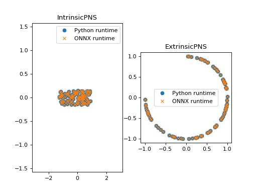
fig = plt.figure()

ax1 = fig.add_subplot(121)
ax1.plot(*int_pns.transform(X).T, "o", label="Python runtime")
ax1.plot(*int_onnx.T, "x", label="ONNX runtime")
ax1.set_xlim(-np.pi, np.pi)
ax1.set_ylim(-np.pi / 2, np.pi / 2)
ax1.legend()
ax1.set_title("IntrinsicPNS")

ax2 = fig.add_subplot(122)
ax2.plot(*ext_pns.transform(X).T, "o", label="Python runtime")
ax2.plot(*ext_onnx.T, "x", label="ONNX runtime")
ax2.set_aspect("equal")
ax2.legend()
ax2.set_title("ExtrinsicPNS")

fig.show()

Module reference

High-level API

class skpns.IntrinsicPNS(n_components=None, tol=0.001, maxiter=None)

Principal nested spheres (PNS) analysis with intrinsic coordinates.

Reduces the dimensionality of data on a high-dimensional hypersphere while preserving its spherical geometry.

The resulting data are intrinsic Euclidean coordinates, which are the scaled residuals in each dimension. For example, n_components=2 represents data on the surface of a 3D sphere.

Parameters:

n_componentsint, default=None

Number of components to keep. Data are transformed onto a Euclidean space in this dimension, representing the surface of a hypersphere with the same dimension. If None, all components are kept, i.e., extrinsic coordinates are converted to intrinsic coordinates without loosing dimenisonality.

tolfloat, default=1e-3

Optimization tolerance.

maxiterint, optional

Maximum number of iterations for the optimization. If None, the number of iterations is not checked.

Attributes:

embedding_ndarray of shape (n_samples, d)

The embedding vectors, \(\Xi(0), \Xi(1), \ldots, \Xi(d-1)\), where the input data is on d-sphere.

v_list of arrays

Principal directions of nested spheres, \(\hat{v}_1, \hat{v}_2, \ldots, \hat{v}_d\).

r_ndarray

Principal radii of nested spheres, \(\hat{r}_1, \hat{r}_2, \ldots, \hat{r}_d\).

Notes

The resulting data is the transposed matrix of

\[\begin{split}\hat{X}_\mathrm{PNS} = \begin{bmatrix} \Xi(0) \\ \Xi(1) \\ \vdots \\ \Xi(n) \end{bmatrix},\end{split}\]

with notations in the original paper, where \(n\) is n_components. The coordinates lie in \([-\pi, \pi] \times [-\pi/2, \pi/2]^{n-1}\), i.e., the azimuthal angle is the first coordinate.

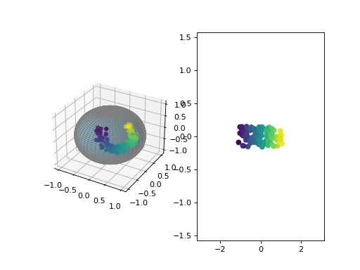
Examples

>>> from skpns import IntrinsicPNS
>>> from skpns.util import circular_data, unit_sphere
>>> X = circular_data()
>>> pns = IntrinsicPNS()
>>> Xi = pns.fit_transform(X)
>>> import matplotlib.pyplot as plt
... fig = plt.figure()
... ax1 = fig.add_subplot(121, projection='3d', computed_zorder=False)
... ax1.plot_surface(*unit_sphere(), color='skyblue', edgecolor='gray')
... ax1.scatter(*X.T, c=Xi[:, 0])
... ax2 = fig.add_subplot(122)
... ax2.scatter(*Xi.T, c=Xi[:, 0])
... ax2.set_xlim(-np.pi, np.pi)
... ax2.set_ylim(-np.pi/2, np.pi/2)

fit(X, y=None)

Find principal nested spheres for the data X.

Parameters:

Xarray-like of shape (n_samples, n_features)

Data on (n_features - 1)-dimensional hypersphere.

yIgnored

Not used, present for API consistency by convention.

Returns:

selfobject

Returns a fitted instance of self.

fit_transform(X, y=None)

Fit the model with data in X and transform X.

Parameters:

Xarray-like of shape (n_samples, n_features)

Data on (n_features - 1)-dimensional hypersphere.

yIgnored

Not used, present for API consistency by convention.

Returns:

X_newarray-like, shape (n_samples, n_components)

X transformed in the new space.

transform(X, y=None)

Transform X onto the fitted subsphere.

Parameters:

Xarray-like of shape (n_samples, n_features)

Data on (n_features - 1)-dimensional hypersphere.

Returns:

X_newarray-like, shape (n_samples, n_components)

X transformed in the new space.

inverse_transform(Xi)

Transform the low-dimensional data back to the original hypersphere.

Parameters:

Xarray-like of shape (n_samples, n_components)

Returns:

X_newarray-like of shape (n_samples, n_features)

Examples

>>> from skpns import IntrinsicPNS
>>> from skpns.util import circular_data, unit_sphere
>>> X = circular_data()
>>> pns = IntrinsicPNS(1)
>>> Xi = pns.fit_transform(X)
>>> X_inv = pns.inverse_transform(Xi)
>>> import matplotlib.pyplot as plt
... ax = plt.figure().add_subplot(projection='3d', computed_zorder=False)
... ax.plot_surface(*unit_sphere(), color='skyblue', edgecolor='gray')
... ax.scatter(*X.T)
... ax.scatter(*X_inv.T)

class skpns.ExtrinsicPNS(n_components=2, tol=0.001, maxiter=None)

Principal nested spheres (PNS) analysis with extrinsic coordinates.

Reduces the dimensionality of data on a high-dimensional hypersphere while preserving its spherical geometry.

The resulting data are represented by extrinsic coordinates. For example, n_components=2 transforms data onto a 2D unit circle, represented by x and y coordinates.

Parameters:

n_componentsint, default=2

Number of components to keep. Data are transformed onto a unit hypersphere embedded in this dimensional space.

tolfloat, default=1e-3

Optimization tolerance.

maxiterint, optional

Maximum number of iterations for the optimization. If None, the number of iterations is not checked.

Attributes:

embedding_ndarray of shape (n_samples, n_components)

Stores the embedding vectors.

v_list of (n_features - 1) arrays

Principal directions of nested spheres.

r_ndarray of shape (n_features - 1,)

Principal radii of nested spheres.

Examples

>>> from skpns import ExtrinsicPNS
>>> from skpns.util import circular_data, unit_sphere
>>> X = circular_data()
>>> pns = ExtrinsicPNS(n_components=2)
>>> X_reduced = pns.fit_transform(X)
>>> X_inv = pns.inverse_transform(X_reduced)
>>> import matplotlib.pyplot as plt
... fig = plt.figure()
... ax1 = fig.add_subplot(121, projection='3d', computed_zorder=False)
... ax1.plot_surface(*unit_sphere(), color='skyblue', alpha=0.6, edgecolor='gray')
... ax1.scatter(*X_inv.T, zorder=10)
... ax1.scatter(*X.T)
... ax2 = fig.add_subplot(122)
... ax2.scatter(*X_reduced.T)
... ax2.set_aspect('equal')

fit(X, y=None)

Find principal nested spheres for the data X.

Parameters:

Xarray-like of shape (n_samples, n_features)

Data on (n_features - 1)-dimensional hypersphere.

yIgnored

Not used, present for API consistency by convention.

Returns:

selfobject

Returns a fitted instance of self.

fit_transform(X, y=None)

Fit the model with data in X and transform X.

Parameters:

Xarray-like of shape (n_samples, n_features)

Data on (n_features - 1)-dimensional hypersphere.

yIgnored

Not used, present for API consistency by convention.

Returns:

X_newarray-like, shape (n_samples, n_components)

X transformed in the new space.

transform(X)

Transform X onto the fitted subsphere.

Parameters:

Xarray-like of shape (n_samples, n_features)

Data on (n_features - 1)-dimensional hypersphere.

Returns:

X_newarray-like, shape (n_samples, n_components)

X transformed in the new space.

inverse_transform(X)

Transform the low-dimensional data back to the original hypersphere.

Parameters:

Xarray-like of shape (n_samples, n_components)

Returns:

X_newarray-like of shape (n_samples, n_features)

to_hypersphere(X)

Alias for inverse_transform().

Low-level functions

Functions for principal nested spheres analysis.

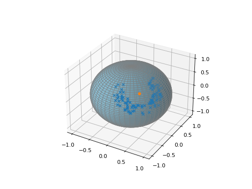
skpns.pns.pss(x, tol=0.001, maxiter=None)

Find the principal subsphere from data on a hypersphere.

Parameters:

x(N, d+1) real array

Extrinsic coordinates of data on a d-dimensional hypersphere, embedded in a d+1-dimensional space.

tolfloat, default=1e-3

Convergence tolerance in radian.

maxiterint, optional

Maximum number of iterations for the optimization. If None, the number of iterations is not checked.

Returns:

v(d+1,) real array

Estimated principal axis of the subsphere in extrinsic coordinates.

rscalar in [0, pi]

Geodesic distance from the pole by v to the estimated principal subsphere.

See also

proj

Project x onto the found principal subsphere.

Notes

This function determines the best fitting subsphere \(\hat{A}_{d-k} = A_{d-k}(\hat{v}_k, \hat{r}_k) \subset S^{d-k+1}\) for \(k = 1, 2, \ldots, d\).

The Fréchet mean \(\hat{A}_0\) of the lowest level best fitting subsphere \(\hat{A}_1\) is also determined by this function.

Examples

>>> from skpns.pns import pss
>>> from skpns.util import circular_data, unit_sphere
>>> x = circular_data()
>>> v, _ = pss(x)
>>> import matplotlib.pyplot as plt
... ax = plt.figure().add_subplot(projection='3d', computed_zorder=False)
... ax.plot_surface(*unit_sphere(), color='skyblue', alpha=0.6, edgecolor='gray')
... ax.scatter(*x.T, marker="x")
... ax.scatter(*v)

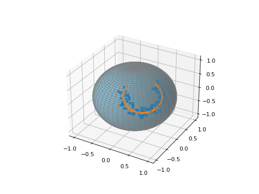
skpns.pns.proj(x, v, r)

Minimum-geodesic projection of points to a subsphere.

Parameters:

x(N, m+1) real array

Extrinsic coordinates of data on a d-dimensional hypersphere, embedded in a d+1-dimensional space.

v(m+1,) real array

Subsphere axis.

rscalar

Subsphere geodesic distance.

Returns:

xP(N, m+1) real array

Extrinsic coordinates of data on a d-dimensional hypersphere, projected onto the found principal subsphere.

res(N, 1) real array

Projection residuals.

See also

pss

Find v and r for the principal subsphere.

embed

Reduce the number of components of the projected data by one.

Notes

This is the function \(P: S^{d-k+1} \to A_{d-k}(v_k, r_k ) \subset S^{d-k+1}\) for \(k = 1, 2, \ldots, d\) in the original paper. Here, \(A_{d-k}(v_k, r_k)\) is a subsphere of the hypersphere \(S^{d-k+1}\). The input and output data dimension are \(m+1\), where \(m = d-k+1\).

This function projects the data onto any subsphere. To project to the principal subsphere \(\hat{A}_{d-k} = A_{d-k}(\hat{v}_k, \hat{r}_k)\), pass the results from pss().

The resulting points have same number of components but their rank is reduced by one in the manifold. Use embed() to further map \(x \in A_{d-k}(v_k, r_k) \subset S^{d-k+1}\) to \(x^\dagger \in S^{d-k}\).

Examples

>>> from skpns.pns import pss, proj
>>> from skpns.util import circular_data, unit_sphere
>>> x = circular_data()
>>> A, _ = proj(x, *pss(x))
>>> import matplotlib.pyplot as plt
... ax = plt.figure().add_subplot(projection='3d', computed_zorder=False)
... ax.plot_surface(*unit_sphere(), color='skyblue', alpha=0.6, edgecolor='gray')
... ax.scatter(*x.T, marker="x")
... ax.scatter(*A.T, marker=".")

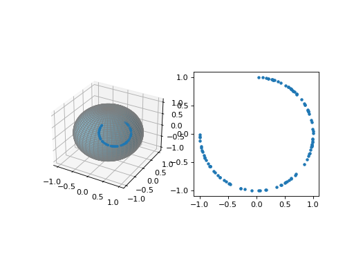
skpns.pns.embed(x, v, r)

Embed data on a sub-hypersphere to a low-dimensional unit hypersphere.

Parameters:

x(N, m+1) real array

Data \(x \in A_{m-1} \subset S^m \subset \mathbb{R}^{m+1}\), on a subsphere \(A_{m-1}\) of a unit hypersphere \(S^m\).

v(m+1,) real array

Sub-hypersphere axis.

rscalar

Sub-hypersphere geodesic distance.

Returns:

(N, m) real array

Data \(x^\dagger\) on a low-dimensional unit hypersphere \(S^{m-1}\).

See also

pss

Find v and r for the principal subsphere.

proj

Project data on a principal subsphere.

reconstruct

Inverse operation of this function.

Notes

This is the function \(f_k: A_{d-k}(v_k, r_k) \subset S^{d-k+1} \to S^{d-k}\) for \(k = 1, 2, \ldots, d-1\) in the original paper. Here, \(A_{d-k}(v_k, r_k)\) is a subsphere of the hypersphere \(S^{d-k+1}\). The input is \(x \in S^m \subset \mathbb{R}^{m+1}\) and the output is \(x^\dagger \in S^{m-1} \subset \mathbb{R}^{m}\), where \(m = d-k+1\).

Examples

>>> from skpns.pns import pss, proj, embed
>>> from skpns.util import circular_data, unit_sphere
>>> x = circular_data()
>>> v, r = pss(x)
>>> A, _ = proj(x, v, r)
>>> A_low = embed(A, v, r)
>>> import matplotlib.pyplot as plt
... fig = plt.figure()
... ax1 = fig.add_subplot(121, projection='3d', computed_zorder=False)
... ax1.plot_surface(*unit_sphere(), color='skyblue', alpha=0.6, edgecolor='gray')
... ax1.scatter(*A.T, marker=".", zorder=10)
... ax2 = fig.add_subplot(122)
... ax2.scatter(*A_low.T, marker=".", zorder=10)
... ax2.set_aspect("equal")

skpns.pns.to_unit_sphere(x, v, r)

alias of embed().

skpns.pns.reconstruct(x, v, r)

Reconstruct data on a low-dimensional unit hypersphere. to a sub-hypersphere.

Parameters:

x(N, m) real array

Data \(x^\dagger\) on a low-dimensional unit hypersphere \(S^{m-1}\).

v(m+1,) real array

Sub-hypersphere axis.

rscalar

Sub-hypersphere geodesic distance.

Returns:

(N, m+1) real array

Data \(x \in A_{m-1} \subset S^m \subset \mathbb{R}^{m+1}\), on a subsphere \(A_{m-1}\) of a unit hypersphere \(S^m\).

See also

embed

Inverse operation of this function.

Notes

This is the function \(f^{-1}_k: S^{d-k} \to A_{d-k}(v_k, r_k) \subset S^{d-k+1}\) for \(k = 1, 2, \ldots, d-1\) in the original paper. Here, \(A_{d-k}(v_k, r_k)\) is a subsphere of the hypersphere \(S^{d-k+1}\). The input is \(x^\dagger \in S^{m-1} \subset \mathbb{R}^{m}\) and the output is \(x \in S^m \subset \mathbb{R}^{m+1}\), where \(m = d-k+1\).

Examples

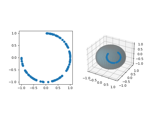
>>> from skpns.pns import reconstruct
>>> from skpns.util import circular_data, unit_sphere
>>> x = circular_data(dim=2)
>>> v = np.array([1 / np.sqrt(3), -1 / np.sqrt(3), 1 / np.sqrt(3)])
>>> r = 0.15 * np.pi
>>> x_high = reconstruct(x, v, r)
>>> import matplotlib.pyplot as plt
... fig = plt.figure()
... ax1 = fig.add_subplot(121)
... ax1.scatter(*x.T)
... ax1.set_aspect("equal")
... ax2 = fig.add_subplot(122, projection='3d', computed_zorder=False)
... ax2.plot_surface(*unit_sphere(), color='skyblue', alpha=0.6, edgecolor='gray')
... ax2.scatter(*x_high.T)

skpns.pns.from_unit_sphere(x, v, r)

alias of reconstruct().

skpns.pns.pns(x, tol=0.001, residual='none', maxiter=None)

Principal nested spheres analysis.

Parameters:

x(N, d+1) real array

Data on a d-sphere.

tolfloat, default=1e-3

Convergence tolerance in radians.

residual{‘none’, ‘scaled’, ‘unscaled’}

If ‘none’, do not yield residuals. If ‘scaled’, yield scaled residuals \(\Xi\). If ‘unscaled’, yield unscaled residuals \(\xi\).

maxiterint, optional

Maximum number of iterations for the optimization. If None, the number of iterations is not checked.

Yields:

v(d+1-i,) real array

Estimated principal axis \(\hat{v}\).

rscalar

Estimated principal geodesic distance \(\hat{r}\).

xd(N, d-i) real array

Transformed data \(x^\dagger\) on low-dimensional unit hypersphere.

res(N,) real array

Residuals. See the description of parameter residual.

See also

reconstruct

Reconstruct the transformed data onto higher-dimensional spheres.

Notes

The input data is \(x \in S^d \subset \mathbb{R}^{d+1}\).

At \(k\)-th iteration for \(k=1, \ldots, d\), this generator yields:

1. The principal axis \(\hat{v}_{k} \in S^{d-k+1} \subset \mathbb{R}^{d-k+2}\),

2. The principal geodesic distance \(\hat{r}_k \in \mathbb{R}\), and

3. The embedded data \(x_k^\dagger \in S^{d-k} \subset \mathbb{R}^{d-k+1}\).

4. (Optional) Scaled residual \(\Xi(d-k)\), or unscaled residual \(\xi_{d-k}\).

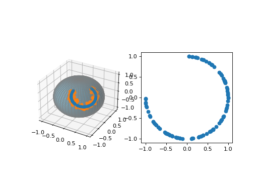
Data projected onto each principal nested sphere in the original space, \(\hat{\mathfrak{A}}_{d-k} \subset S^d\), can be found by recursively calling reconstruct() on \(x_k^\dagger\).

Examples

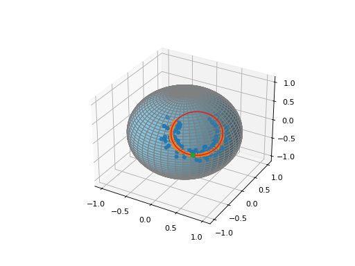
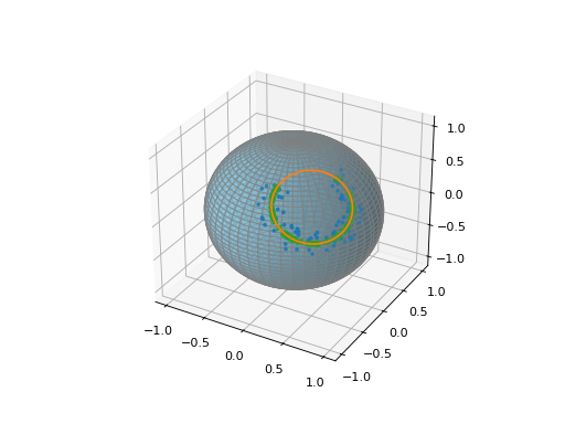
Use reconstruct() to map reduced data onto the original sphere.

>>> from skpns.pns import pns, reconstruct
>>> from skpns.util import circular_data, unit_sphere, circle
>>> x = circular_data()
>>> pns_gen = pns(x, residual="none")
>>> v1, r1, xd1 = next(pns_gen)
>>> v2, r2, xd2 = next(pns_gen)
>>> import matplotlib.pyplot as plt
... ax = plt.figure().add_subplot(projection='3d', computed_zorder=False)
... ax.plot_surface(*unit_sphere(), color='skyblue', edgecolor='gray')
... ax.scatter(*x.T)
... ax.scatter(*reconstruct(xd1, v1, r1).T, marker="x")
... ax.scatter(*reconstruct(reconstruct(xd2, v2, r2), v1, r1).T, zorder=10)
... ax.plot(*circle(v1, r1), color="tab:red")

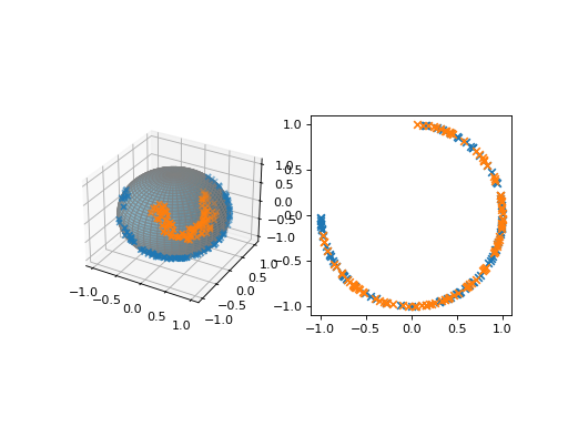
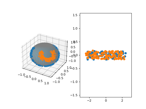
Unscaled residuals do not distinguish the scale of the data on the original sphere.

>>> X = circular_data(scale="large")
>>> (V1, R1, XD1, XI1), (V2, R2, XD2, XI2) = list(pns(X, residual="unscaled"))
>>> x = circular_data(scale="small")
>>> (v1, r1, xd1, xi1), (v2, r2, xd2, xi2) = list(pns(x, residual="unscaled"))
>>> fig = plt.figure()
... ax1 = fig.add_subplot(121, projection='3d', computed_zorder=False)
... ax1.plot_surface(*unit_sphere(), color='skyblue', edgecolor='gray')
... ax1.scatter(*X.T)
... ax1.scatter(*x.T)
... ax2 = fig.add_subplot(122)
... ax2.scatter(XI2, XI1)
... ax2.scatter(xi2, xi1)
... ax2.set_xlim(-np.pi, np.pi)
... ax2.set_ylim(-np.pi/2, np.pi/2)

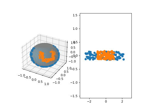
Scaled residuals distinguish different arc-lengths of principal subspheres.

>>> X = circular_data(scale="large")
>>> (V1, R1, XD1, XI1), (V2, R2, XD2, XI2) = list(pns(X, residual="scaled"))
>>> x = circular_data(scale="small")
>>> (v1, r1, xd1, xi1), (v2, r2, xd2, xi2) = list(pns(x, residual="scaled"))
>>> fig = plt.figure()
... ax1 = fig.add_subplot(121, projection='3d', computed_zorder=False)
... ax1.plot_surface(*unit_sphere(), color='skyblue', edgecolor='gray')
... ax1.scatter(*X.T)
... ax1.scatter(*x.T)
... ax2 = fig.add_subplot(122)
... ax2.scatter(XI2, XI1)
... ax2.scatter(xi2, xi1)
... ax2.set_xlim(-np.pi, np.pi)
... ax2.set_ylim(-np.pi/2, np.pi/2)

skpns.pns.Exp(z)

Exponential map of hypersphere at (0, 0, …, 0, 1).

Parameters:

z(N, d) real array

Vectors on tangent space.

Returns:

(N, d+1) real array

Points on d-sphere.

skpns.pns.Log(x)

Log map of hypersphere at (0, 0, …, 0, 1).

Parameters:

x(N, d+1) real array

Points on d-sphere.

Returns:

(N, d) real array

Vectors on tangent space.

Utilities

Utility functions for data generation and transformation.

skpns.util.circular_data(dim=3, scale='small')

Circular data on a 3D unit sphere, or its projection to 2D unit sphere.

Parameters:

dim{3, 2}

Data dimension.

scale{“small”, “large”}

Size of the circle around the 3D sphere.

Returns:

ndarray of shape (100, dim)

Data coordinates.

Examples

Note how data occupy different scales in 3D, but their projection onto each principal subsphere is identical.

>>> from skpns.util import circular_data, unit_sphere
>>> import matplotlib.pyplot as plt
... fig = plt.figure()
... ax1 = fig.add_subplot(121, projection='3d', computed_zorder=False)
... ax1.plot_surface(*unit_sphere(), color='skyblue', alpha=0.6, edgecolor='gray')
... ax1.scatter(*circular_data(3, scale="large").T, marker="x")
... ax1.scatter(*circular_data(3, scale="small").T, marker="x")
... ax2 = fig.add_subplot(122)
... ax2.scatter(*circular_data(2, scale="large").T, marker="x")
... ax2.scatter(*circular_data(2, scale="small").T, marker="x")
... ax2.set_aspect("equal")

skpns.util.unit_sphere()

Helper function to plot a unit sphere.

Returns:

x, y, zarray

Coordinates for unit sphere.

skpns.util.circle(v, theta, n=100)

Helper function to plot a circle in 3D.

Parameters:

v(3,) array

Unit vector to center of circle in 3D.

thetascalar

Geodesic distance.

nint, default=100

Number of points.